Fitting Light Curves (with SALT2)
Light curve fitting in SNANA uses the snlc_fit.exe
program with a FORTRAN namelist file to provide paramers.
It’s easy enough to write, though a bit idiosyncratic
(comments, for example, are exclamation marks).
I’m going to focus on fitting the SALT2 model here,
which is the standard approach for most analyses.
But SNANA can fit light curves using some of the other models
in the $SNDATA_ROOT/models directory such as
MLCS and SNooPy, for exampe.
Writing the Namelist (NML) File
The snlc_fit.exe namelist has
three sections. First, the header section,
which is only really used when running in
batch mode (discussed briefly below).
Next, the SNLCINP section,
generally the SN light curve input
parameters and the FITINP
section, for the fitting input parameters.
The lines discussed below will be written to
a file called snfit_PS1.NML.
The SNLCINP section
The SNLCINP section is bracketed by:
&SNLCINP

   ! a bunch of options here

&END
First, some options to find the input files, the filters, and which LC files to read in:
VERSION_PHOTOMETRY = 'PS1MD' ! name of your simulation or real data
KCOR_FILE          = '../kcor/kcor_PS1.fits' ! kcor file we made earlier
Basic outputs:
SNTABLE_LIST     = 'SNANA FITRES(text:key)' ! this is standard output format
TEXTFILE_PREFIX  = 'PS1MD' ! output filename (w/o the extension)
Milky Way reddening:
RV_MWCOLORLAW = 3.1
OPT_MWCOLORLAW = 99
OPT_MWEBV = 1
These lines give the value of R_V
for the Milky Way, the Milky Way reddening
colorlaw (99 = Fitzpatrick 1999), and
OPT_MWEBV = ` means `snlc_fit will
correct the light curves for MW reddening
before fitting.
One CUTWIN option:
CUTWIN_REDSHIFT = 0.02, 1.0
The syntax here is that CUTWIN_ followed
by any variable can be used to make cuts (min,max)
on the input light curves.
Then there are a few fit options that appear
to not be placed in the FITINP section for
reasons I don’t totally understand:
NFIT_ITERATION = 3
INTERP_OPT     = 1
ABORT_ON_NOEPOCHS = F
LDMP_SNFAIL = T
Number of fitting iterations, the interpolation option (1 = linear interpolation), avoid aborting just because a SN cannot be fit, and report the reason for each SN that fails.
The FITINP section
Next, the fit options. Same as before, the section is denoted with:
&FITINP

   ! a bunch of options

&END
Then, identify the model and filter set:
FITMODEL_NAME  = 'SALT2.JLA-B14'
FILTLIST_FIT = 'griz'
This is SALT2.4, from Betoule et al. (2014). In a perfect
world, you would know this from reading
$SNDATA_ROOT/models/SALT2/SALT2.JLA-B14/AAA_README.
However, in this case you’ll have to just trust me.
Next, a prior on the time of maximum light and a window defining the range of rest-frame times (relative to peak) to include:
PRIOR_MJDSIG        = 25.0
TREST_REJECT  = -15.0, 45.0
And a few more things:
LFIXPAR_ALL     = F
OPT_COVAR = 1
OPT_COVAR_MWXTERR = 1
FUDGEALL_ITER1_MAXFRAC = 0.02
These just say, don’t fix all the parameters, do use a model covariance matrix, do use Milky Way reddening uncertainty in the covariance matrix, and inflate the uncertainties by 2% for the first fitting iteration only.
That’s it!
Analyzing the Output
Recent versions of SNANA have cleaned up the
output format a bit so that output files are
easier to parse. The FITRES ASCII format gives
a line starting with VARNAMES that identifies
all the variables and subsequent lines starting with
SN for the light curve parameters, metadata,
and covariances.
Plotting light curves with their corresponding SALT2 fits however, is not (in my opinion) very intuitive. I usually resort to sncosmo and a custom script (below).
Plotting Light Curve Fits
I’ve included a clumsy python script, txtobj.py
for reading FITRES files. But, it’s easy enough to make
your own, or use astropy utilities instead.
To read in the output FITRES file and generate a basic light curve plot like we had before in the simulations guide, first the basic imports:
import glob
import os
import matplotlib.pyplot as plt
import numpy as np
from util import snana
from util.txtobj import txtobj
And then a few lines to read/plot stuff:
fr = txtobj('fitting/PS1MD.FITRES.TEXT',fitresheader=True)

lcfiles = glob.glob(os.path.expandvars('$SNDATA_ROOT/SIM/PS1MD/*DAT'))
sn = snana.SuperNova(lcfiles[10])
for f in sn.FILTERS:
    plt.errorbar(sn.MJD[sn.FLT == f],sn.FLUXCAL[sn.FLT == f],
                 yerr=sn.FLUXCALERR[sn.FLT == f],label=f,fmt='o')
plt.ylabel('Flux')
plt.xlabel('MJD')
plt.legend()
Now add the parameters from the fit:
iSN = fr.CID == sn.SNID
plt.title('SNID = %s, $x_0$ = %8.2e, $x_1$ = %.2f, c = %.3f'%(
          sn.SNID,fr.x0[iSN],fr.x1[iSN],fr.c[iSN]))

Now plot the SALT model (you’ll need sncosmo for this example):
import sncosmo
from util import register

dust = sncosmo.F99Dust()
dust.set(ebv=float(sn.MWEBV.split()[0])) # pretty ugly but whatever

model = sncosmo.Model(source='salt2',effects=[dust],effect_names=['mwebv'],effect_frames=['obs'])
# NOTE - SNANA SALT2 implementation has a 0.27 mag offset from sncosmo.
# this doesn't matter at all for most things like cosmology analyses,
# but certainly matters for making plots
model.set(z=fr.zHEL[iSN],t0=fr.PKMJD[iSN],
          x1=fr.x1[iSN],c=fr.c[iSN],x0=fr.x0[iSN]*10**(-0.4*(0.27)))

# register the filters to sncosmo using the kcor file.  sncosmo has
# pre-canned filter sets but it's best to be safe in a game where mmag
# offsets matter
mjd = np.arange(fr.PKMJD[iSN]-40,fr.PKMJD[iSN]+80,1)
register.from_kcor('kcor/kcor_PS1.fits')
for i,f in enumerate(sn.FILTERS):

    # careful about zpsys!
    salt2flux = model.bandflux(f, mjd, zp=27.5, zpsys='AB')
    plt.plot(mjd,salt2flux,color='C%i'%i)
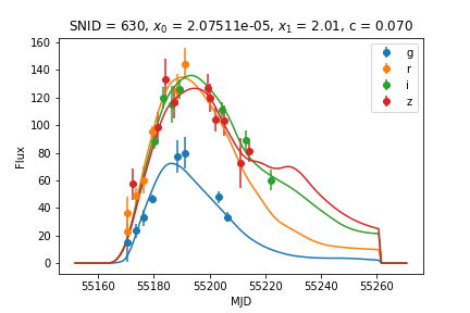
An important caveat - sncosmo won’t check whether your filters are too red or blue for the SALT2 model. If your central filter wavelength in the SN rest frame is redder than 7000 Angstroms or bluer than 2800 Angstroms then SNANA did not include it in the fit!
Generating Distances and Making a Quick Hubble Diagram
More sophisticated ways of getting distances are discussed in the distances section, but for a small sample it’s OK to use a simpler method. Namely, plugging light curve parameters into the Tripp formula and grabbing nuisance parameters from the latest and greatest cosmological analysis (at the time of writing, Scolnic et al. 2018).
The Tripp formula (Tripp 1999), to compute distance modulus \(\mu\)
I’m excluding the mass step for these purposes, as well as things like bias corrections. Nuisance parameter M is approximately -19.36 for \(H_0 = 70\) km s:math:^{-1} Mpc:math:^{-1}, while nuisance parameters \(\alpha\) and \(beta\) are xxx and yyy from the Pantheon analysis (non-bias corrected version).
This is simple in Python, but the errors have to take
the covariances into account. I included a script getmu.py
that does the work.
Making a Hubble diagram is pretty easy then:
# import our baseline cosmological params for comparison
from astropy.cosmology import Planck15 as cosmo
from util import getmu

# gives the fitres object a "mu", "muerr" and "mures" attribute
fr = getmu.getmu(fr)
fr = getmu.mkcuts(fr)
iErr = fr.muerr < 0.2 # no crazy errors!

zrange = np.arange(0,1,0.01)
plt.plot(zrange,cosmo.distmod(zrange).value,color='k')
plt.errorbar(fr.zCMB[iErr],fr.mu[iErr],yerr=fr.muerr[iErr],fmt='o')
plt.xlabel('$z_{CMB}$',fontsize=15)
plt.ylabel('$\mu$',fontsize=15)
plt.xlim([0.05,0.6])
plt.ylim([36,44])
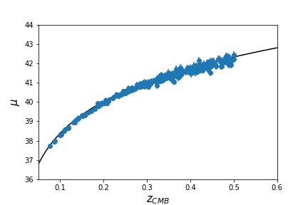
Note the SNe fall a little bit below the \(\Lambda\)CDM line. That’s ok, it’s just an artifact of \(H_0\) and the SN absolute magnitude being degenerate. We marginalize over this global offset in cosmological analyses.
Done!
Running in Batch Mode
Check back later!
Please report any issues with this guide using the SNANA_StarterKit GitHub page.