Running a Simple Simulation
SNANA is an extremely powerful tool for survey simulations, and can simulate nearly every aspect of a survey, at least on the catalogue level (not pixel level) that I can think of.
From Kessler et al. (2019), here’s a basic schematic of the SNANA simulation framework.
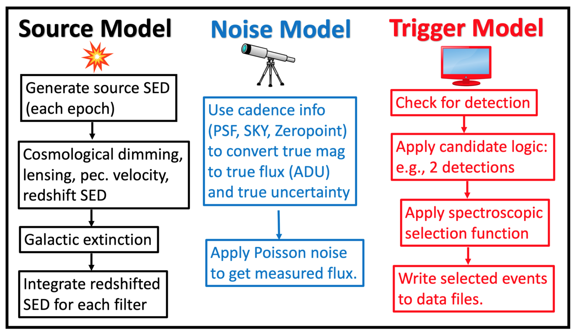
Building a SNANA simulation requires at minimum,
four principal files: the KCOR file,
the SIMLIB file, which contains the
sequence of observations to simulate, the SEARCHEFF
file that gives the efficiency of SN detection, and finally
the sim-input file which is passed to the simulation
program, snlc_sim.exe.
Writing a Simple SIMLIB File
The SIMLIB file defines the parameters of the survey observations. At minimum, this requires a list of MJDs, filters, sky noise, and image zeropoints. Here is a brief example for the Pan-STARRS medium deep survey:
TELESCOPE: PS1
SURVEY: PS1MD    FILTERS: griz

BEGIN LIBGEN  2016-3-28
# --------------------------------------------
LIBID: 1
RA: 0    DECL: 0 NOBS: 6 MWEBV: 0.024   PIXSIZE: 0.25
FIELD: 1
#                           CCD  CCD         PSF1 PSF2 PSF2/1
#     MJD      IDEXPT  FLT GAIN NOISE SKYSIG (pixels)  RATIO  ZPTAVG ZPTERR  MAG
S: 55074.600 0 g 1.0 0.0 6.8691 3.7960 0.0000 0.0000 30.2426 0.0034 -99
S: 55086.600 1 g 1.0 0.0 10.319 4.4315 0.0000 0.0000 30.1481 0.0034 -99
S: 55089.600 2 g 1.0 0.0 6.8671 2.8140 0.0000 0.0000 30.2175 0.0036 -99
S: 55095.500 3 g 1.0 0.0 7.2529 3.9464 0.0000 0.0000 30.3894 0.0041 -99
S: 55098.500 4 g 1.0 0.0 6.8112 3.3349 0.0000 0.0000 30.1146 0.0040 -99
S: 55101.600 5 g 1.0 0.0 7.4172 3.1407 0.0000 0.0000 30.1131 0.0037 -99
END_LIBID: 1
END_OF_SIMLIB: 1 ENTRIES
The basic syntax here is a short header, where the
TELESCOPE and SURVEY keys shouldn’t have
any impact on the simulated outputs and FILTERS is
just the list of one-letter filter names (specified in your
KCOR file).
Next, there are a couple lines that specify different “libraries” with
the LIBID key. In this case, LIBID or FIELD
can serve to separate the simulation into distinct groups where simulated
supernovae do not overlap.
The keys RA, DEC, NOBS, MWEBV, and
PIXSIZE are right ascension, declination, number of
observations, Milky Way E(B-V), and the pixel size of the detector.
In particular, the pixel size of the detector is important for
generating simulations with realistic noise properties.
Now, the observation lines:
#                           CCD  CCD         PSF1 PSF2 PSF2/1
#     MJD      IDEXPT  FLT GAIN NOISE SKYSIG (pixels)  RATIO  ZPTAVG ZPTERR  MAG
S: 55074.600 0 g 1.0 0.0 6.8691 3.7960 0.0000 0.0000 30.2426 0.0034 -99
In order, these fields are the observed MJD, an integer label for the observation number, the filter, the gain, the CCD noise (I think this is read noise?) and the RMS of the sky measurements. Next, three parameters of the PSF, which are spread in X, spread in Y, and the ratio of the two. Those second parameters can be set to 0 and SNANA will assume a spherically symmetric PSF.
ZPTAVG is the image zeropoint and the ZPTERR will be
propagated to the observational uncertainties. MAG should
be set to -99 or else SNANA will simulate only those specific magnitudes on
a given date.
The Search-Efficiency File
The search-efficiency file defines the probability of detecting a source as a function of magnitude. This file is a essentially a two-column list for one or multiple filters that gives a magnitude and a probability of detection. Here’s an example:
PHOTFLAG_DETECT: 4096
FILTER: g
SNR:  0.500  0.001
SNR:  1.500  0.004
SNR:  2.500  0.028
SNR:  3.500  0.189
SNR:  4.500  0.428
SNR:  5.500  0.644
SNR:  6.500  0.796
SNR:  7.500  0.841
SNR:  8.500  0.949
SNR:  9.500  0.861
SNR:  10.500  0.936
SNR:  11.500  0.956
SNR:  12.500  0.952
SNR:  13.500  0.920
SNR:  14.500  1.000
SNR:  15.500  1.000
SNR:  16.500  0.857
SNR:  17.500  0.933
SNR:  18.500  1.000
SNR:  19.500  1.000
FILTER: r
SNR:  0.500  0.001
SNR:  1.500  0.004
SNR:  2.500  0.025
SNR:  3.500  0.177
SNR:  4.500  0.423
SNR:  5.500  0.593
SNR:  6.500  0.693
SNR:  7.500  0.769
SNR:  8.500  0.878
SNR:  9.500  0.850
SNR:  10.500  0.900
SNR:  11.500  0.871
SNR:  12.500  0.849
SNR:  13.500  0.915
SNR:  14.500  0.969
SNR:  15.500  0.860
SNR:  16.500  0.889
SNR:  17.500  0.952
SNR:  18.500  0.864
SNR:  19.500  0.955
PHOTFLAG_DETECT is just a value that is added to the simulated
data file to indicate whether or not a given epoch was high enough
SNR to be “detected” in the simulation.
The SEARCHEFF_PIPELINE_LOGIC_FILE
This one is pretty simple. The pipeline logic file tells the simulation what combination of individual detections in various filters and epochs constitutes a “detection” for the purposes of the survey. For example, detections in two different filters or two separate detections.
Here are a couple examples. For a survey that requires two detections in any one of griz:
PS1MD: 2 g+r+i+z # require 1 epoch, any band
Here’s SDSS:
SDSS: 3 gr+ri+gi # require 3 epochs, each with detection in two bands.
The Sim-Input File
Finally, the input file! Starting with the basics:
GENVERSION: PS1MD         # simname
GENSOURCE:  RANDOM
GENMODEL:   SALT2.JLA-B14
GENPREEFIX: YSE_IA
RANSEED: 128473       # random number seed

SIMLIB_FILE: PS1MD_test.simlib # simlib file

KCOR_FILE:  kcor_PS1.fits
GENVERSION is the name of the simulation, GENSOURCE
can be set to RANDOM or GRID. GRID simulations are a whole
thing - let’s stick to RANDOM (Monte Carlo) simulations.
GENMODEL refers to one of the “model” directories in
$SNDATA_ROOT/models.
SNANA has kind of a peculiar
way of identifying models. The first word (before the period)
specifies the model type while the portion after the period
specifies the version. In this case, SALT2.B14
is SALT2.4 from Betoule et al. (2014), but extrapolated to
slightly redder wavelengths than the original model.
The model directory is $SNDATA_ROOT/models/SALT2/SALT2.JLA-B14
and some additional information is in the SALT2.INFO file in that
directory. Some models also have README files, which are helpful :).
Onwards! There are three ways to figure out how many
SNe to simulate (that I’m aware of). The first is NGEN_LC, which
tells the simulation to run until the specified number
of SNe have been detected and pass all cuts. The second
is NGENTOT_LC, which tells the simulation to
run until the specified number of SNe have been simulated
regardless of whether or not they pass cuts.
The third option is NGEN_SEASON which uses the catalog of
observations, the SOLID_ANGLE key , and the SN rates
to figure out how many SNe your survey is expected to observe:
NGEN_LC: 5000

APPLY_SEARCHEFF_OPT: 1

EXPOSURE_TIME_FILTER: g 1.0
EXPOSURE_TIME_FILTER: r 1.0
EXPOSURE_TIME_FILTER: i 1.0
EXPOSURE_TIME_FILTER: z 1.0

GENFILTERS: griz

GENSIGMA_SEARCH_PEAKMJD:  1.0 # sigma-smearing for  SEARCH_PEAKMJD (days)

GENRANGE_PEAKMJD:  55000 56000
SOLID_ANGLE: 0.192
APPLY_SEARCHEFF_OPT set to 1 keeps all
“detected” SNe, but does not require that a SN has
spectroscopic confirmation (APPLY_SEARCHEFF_OPT = 3)
or a host galaxy redshift (APPLY_SEARCHEFF_OPT = 5)
- those can be specified in more complicated simulations.
APPLY_SEARCHEFF_OPT = 0 can be used to keep
all SNe, detected or not.
EXPOSURE_TIME_FILTER here is set to 1.0, which
just uses the nominal zeropoints, etc specified in the
SIMLIB file. It can be scaled up or down to easily adjust
simulations.
GENSIGMA_SEARCH_PEAKMJD just adds uncertainty
to the time of maximum light reported in the generated
file headers.
Next, referencing the search efficiency files:
SEARCHEFF_PIPELINE_FILE:  SEARCHEFF_PIPELINE_PS1.DAT
SEARCHEFF_PIPELINE_LOGIC_FILE:  SEARCHEFF_PIPELINE_LOGIC_PS1.DAT
Then, the redshift range to simulate. the redshift uncertainty to simulate, and the range of time around maximum light that is simulated for each light curve:
GENRANGE_REDSHIFT:  0.01    0.5
GENSIGMA_REDSHIFT:  0.000001
GENRANGE_TREST:   -20.0    80.0     # rest epoch relative to peak (days)
Next, SN rates. There are a lot of options here, but for low-z simulations a simple power law will suffice:
DNDZ: POWERLAW 2.6E-5 2.2 # rate=2.6E-5*(1+z)^1.5 /yr/Mpc^3
Here’s an alternate example with two power laws from the manual:
# R0 Beta Zmin Zmax
DNDZ: POWERLAW2 2.2E-5 2.15 0.0 1.0 # rate = R0(1+z)^Beta
DNDZ: POWERLAW2 9.76E-5 0.0 1.0 2.0 # constant rate for z>1
And some extra things:
OPT_MWEBV: 1 # simulate galactic extinction from values in SIMLIB file

# smear flags: 0=off, 1=on
SMEARFLAG_FLUX:    1  # photo-stat smearing of signal, sky, etc ...
SMEARFLAG_ZEROPT:  1  # smear zero-point with zptsig
Apply some sample cuts:
APPLY_CUTWIN_OPT:     1
CUTWIN_NEPOCH:   5 -5.              # require 5 epochs (no S/N requirement)
CUTWIN_TRESTMIN: -20  10
CUTWIN_TRESTMAX:   9  40
CUTWIN_MWEBV:      0 .20
CUTWIN_SNRMAX:   5.0 griz 2 -20. 80.  # require 1 of griz with S/N > 5
FORMAT_MASK: 32 specifies FITS format, while FORMAT_MASK: 2
is ASCII:
FORMAT_MASK: 2 # terse format
Parameters of the SALT model:
# SALT shape and color parameters
GENMEAN_SALT2x1:     0.703
GENRANGE_SALT2x1:   -5.0  +4.0     # x1 (stretch) range
GENSIGMA_SALT2x1:    2.15  0.472      # bifurcated sigmas

GENMEAN_SALT2c:     -0.04
GENRANGE_SALT2c:   -0.4   0.4     # color range
GENSIGMA_SALT2c:    0.033   0.125     # bifurcated sigmas
Nuisance parameters from the Tripp formula. Alpha is the correlation of shape parameter x1 with distance, while Beta is the correlation of color parameter c with distance.:
# SALT2 alpha and beta
GENMEAN_SALT2ALPHA:   0.14
GENMEAN_SALT2BETA:   3.1
Cosmological parameters:
# cosmological params for lightcurve generation and redshift distribution
OMEGA_MATTER:  0.3
OMEGA_LAMBDA:  0.7
W0_LAMBDA:    -1.00
H0:            70.0
And last but not least, variables to “dump” to an output file for every SN (not just those detected). The first number is the number of variables:
SIMGEN_DUMPALL: 10 CID Z PEAKMJD S2c S2x1 SNRMAX MAGT0_r MAGT0_g MJD_TRIGGER NON1A_INDEX
The SIMGEN_DUMPALL key will save the specified columns for both detected and undetected SNe, while SIMGEN_DUMP will save the information only for detected SNe. The full example file is available here.
Core-collapse and other non-Ia Simulations
For non-Ia simulations, only a couple things need to be changed in the input file:
GENMODEL:   NON1A
DNDZ: POWERLAW2 5E-5   4.5   0.0   0.8    # rate = R0(1+z)^Beta for z<0.8
DNDZ: POWERLAW2 5.44E-4  0.0   0.8   9.1  # rate = constant for z>0.8
DNDZ_PEC1A: POWERLAW  2.6E-5  2.2

INPUT_FILE_INCLUDE: $SNDATA_ROOT/snsed/NON1A/SIMGEN_INCLUDE_NON1A_J17-beforeAdjust.INPUT
These lines change the generated model, the SN rates (including a new term for peculiar SNe Ia), and add an input file that defines the contribution of different CC SN templates.
Running the Simulation
Now that the files are assembled, running the simulations is easy:
snlc_sim.exe sim_PS1.input
The default output is placed in $SNDATA_ROOT/SIM.
For your first simulation, you may need to execute
the following command before running the simulation:
mkdir $SNDATA_ROOT/SIM
Examining the Output
Basic properties from the DUMP file
The simulated light curves are located in
$SNDATA_ROOT/SIM/<genversion/. First,
notice the *.DUMP file, which contains
the variables specified in the SIMGEN_DUMP
variable in your sim-input file. This is a good
way to get some overview statistics for your sample.
For example, plotting the redshift and peak mag distribution of your simulation. Starting with some imports:
import numpy as np
import os
import matplotlib.pyplot as plt
from txtobj import txtobj

# read in the DUMP file
dmp = txtobj(os.path.expandvars('$SNDATA_ROOT/SIM/PS1MD/PS1MD.DUMP'),fitresheader=True)
print(dmp.__dict__.keys())
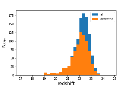
Plotting a redshift histogram for detected and undetected SNe:
bins = np.arange(0,0.55,0.05)
plt.hist(dmp.Z,label='all',bins=bins)
plt.hist(dmp.Z[dmp.MJD_TRIGGER != 1000000.000],bins=bins,label='detected')
plt.ylabel('N$_{SNe}$',fontsize=15)
plt.xlabel('redshift',fontsize=15)
plt.legend()

Plotting a peak magnitude distribution:
bins = np.arange(17,25,0.25)
plt.hist(dmp.MAGT0_r,label='all',bins=bins)
plt.hist(dmp.MAGT0_r[dmp.MJD_TRIGGER != 1000000.000],bins=bins,label='detected')
plt.ylabel('N$_{SNe}$',fontsize=15)
plt.xlabel('redshift',fontsize=15)
plt.legend()
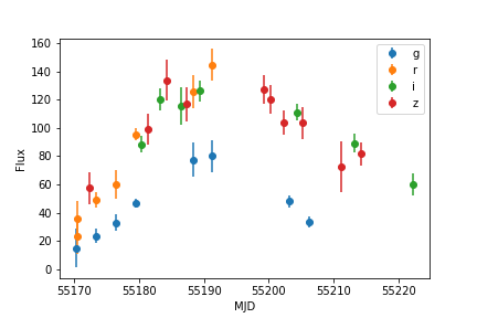
The Simulated Light Curves
Let’s take a look at some of the simulated ASCII files. These can be easily parsed with the snana.py script in the utils directory:
import numpy as np
import snana
import matplotlib.pyplot as plt
import os
import glob

lcfiles = glob.glob(os.path.expandvars('$SNDATA_ROOT/SIM/PS1MD/*DAT'))
sn = snana.SuperNova(lcfiles[10])
for f in sn.FILTERS:
    plt.errorbar(sn.MJD[sn.FLT == f],sn.FLUXCAL[sn.FLT == f],
                 yerr=sn.FLUXCALERR[sn.FLT == f],label=f,fmt='o')
plt.ylabel('Flux')
plt.xlabel('MJD')
plt.legend()
In FITS format, things are a little bit more annoying. Luckily, the LCs can be converted to a PANDAS dataframe thanks to some utilities from the PLAsTiCC team and Alexandre Boucaud (I modified them slightly).
As a reminder, use FORMAT_MASK: 32 in your sim-input file
to use FITS format and FORMAT_MASK: 2 for ASCII format.
A quick example for plotting a FITS-format light curve is below:
from sim_serializer import serialize
import matplotlib.pyplot as plt
datadict = serialize.main('PS1MD')
for key in datadict[list(datadict.keys())[20]].keys():
  if key == 'header': continue
  plt.errorbar(datadict[501][key]['mjd'],
              datadict[501][key]['fluxcal'],
              yerr=datadict[501][key]['fluxcalerr'],
              fmt='o',label=key)
plt.ylabel('flux')
plt.xlabel('mjd')
Please report any issues with this guide using the SNANA_StarterKit GitHub page.